Lab 1 - AI Model Design and Quantization

Lab 1.1 - AI Model Design

1. Targeting Task and Dataset

In the labs of this course, we will perform an image classification task on the CIFAR-10 dataset. CIFAR-10 consists of 60,000 colored images (32×32 pixels, RGB channels) across 10 classes: airplane, automobile, bird, cat, deer, dog, frog, horse, ship, and truck. It is split into 50,000 training and 10,000 test images.

Many convolutional neural networks (CNNs) have been evaluated on CIFAR-10, making it a valuable dataset for learning image classification techniques.

2. Model Architecture Design

Below, we introduce several commonly used operators in convolutional neural networks (CNNs). In the assignment of this lab, you will be asked to design your own model architecture using these operators and apply it to the CIFAR-10 image classification task.

In the following formulas, we present:

\[ \begin{align} N &= \text{batch size} \\ C_{\text{in}} &= \text{number of input channels} \\ C_{\text{out}} &= \text{number of output channels} \\ H &= \text{height of the tensor} \\ W &= \text{width of the tensor} \end{align} \]

Convolution

Convolutions are widely used for feature extraction in computer vision tasks. A convolution operator can defined by its size, stride, padding, dilation, etc.

Here is the mathematical representation:

\[ \begin{align} \text{out}(N_i, C_{\text{out}, j}) &= \text{bias}(C_{\text{out}, j}) + \sum_{k=0}^{C_{\text{in}}-1} \text{weight}(C_{\text{out}, j}, k) \star \text{input}(N_i, k) \\ \end{align} \]

In AlexNet, 11×11, 5×5, and 3×3 Conv2D layers are used. However, using multiple convolution kernel sizes in a model increases the complexity of hardware implementation. Therefore, in this lab, we will use only 3×3 Conv2D with a padding size of 1 and a stride of 1, following the approach in VGGNet. With these settings, the spatial dimensions of the output feature map will remain the same as those of the input feature map.

Linear

Fully-connected layers, also known as linear layers or dense layers, connect every input neuron to every output neuron and are commonly used as the classifier in a neural network.

\[ \mathbf{y} = \mathbf{x} \mathbf{W}^{T} + \mathbf{b} \]

Rectified Linear Unit (ReLU)

ReLU is an activation function, which sets all negative values to zero while keeping positive values unchanged. It introduces non-linearity to the model, helping neural networks learn complex patterns while mitigating the vanishing gradient problem compared to other activation functions like sigmoid, hyperbolic tangent, etc.

{width=75%}

\[ \operatorname{ReLU}(x) = \cases{ 0 \text{, if } x < 0 \\ x \text{, otherwise} } \]

Max Pooling

Max pooling is a downsampling operation commonly used in convolutional neural networks (CNNs) to reduce the spatial dimensions of feature maps while preserving important features. In the following formulas, we present the typical 2D max pooling operation.

{width=80%}

\[ out(N_i, C_j, h, w) = \max\limits_{m=0,\dots,k_H-1} \max\limits_{n=0,\dots,k_W-1} \text{input}(N_i, C_j, \text{stride}[0] \times h + m, \text{stride}[1] \times w + n) \]

Batch Normalization

Batch Normalization (BN) is a technique used in deep learning to stabilize and accelerate training by normalizing the inputs of each layer. It reduces internal covariate shift, making optimization more efficient.

\[ \begin{align} y &= \frac{x - \mathbb{E}[x]}{\sqrt{\text{Var}[x] + \epsilon}} \cdot \gamma + \beta \\ \text{where} \\ \mathbb{E}[\cdot] &= \text{"the mean"} \\ \text{Var}[\cdot] &= \text{"the variance"} \\ \gamma, \beta &= \text{"learnable parameters"} \in \mathbb{R}^{C_\text{out}} \\ \epsilon &= \text{"small constant to avoid division by zero"} \\ \end{align} \]

The learnable parameters \(\gamma\) and \(\beta\) are updated during training but remains fixed during inference.

1. During forward propagation of training: the mean and variance are calculated from the current mini-batch.
2. During backward propagation of training: \(\gamma\) and \(\beta\) are updated with the gradients \(\frac{\partial L}{\partial \gamma}\) and \(\frac{\partial L}{\partial \beta}\) respectively
3. During inference: \(\gamma\) and \(\beta\) are fixed

As the following figure shows, the batch normalization are applied per channel. That is, the mean and variance are computed over all elements in the batch (\(N\)) and spatial dimension (\(H\) and \(W\)). Each channel has independent \(\gamma_c\) and \(\beta_c\) parameters.

3. Model Training and Hyperparameter Tuning

You can use these techniques to improve the accuracy and efficiency of model training. - Learning Rate Scheduling and Optimizer - Weight Initialization - Regularization (L1, L2) - Softmax and Cross Entropy Loss - They are commonly used in image classification tasks.

Lab 1.2 - AI Model Quantization

Why Quantization?

In the beginning, we need to discuss the different data types that can be used for computation and their associated hardware costs.

Number Representation

Integers

Integer Format	Length (bit)	Value Range
INT32	32	-2,147,483,648 ~ 2,147,483,647
UINT32	32	0 ~ 4,294,967,295
INT16	16	-32768 ~ 32767
UINT16	16	0 ~ 65535
INT8	8	-128 ~ 127
UINT8	8	0 ~ 255

Floating Point Numbers

Floating Point Format	Length (bits)	Exponent (E)	Mantissa (M)	Applications
FP64	64	11	52	High precision computing, scientific simulations
FP32	32	8	23	General computing, 3D rendering, machine learning
TF32	32	8	10	NVIDIA proposed, AI training acceleration
FP16	16	5	10	Low-power AI training and inference
BF16	16	8	7	AI training, better compatibility with FP32
FP8-E4M3	8	4	3	Low-precision AI inference
FP8-E5M2	8	5	2	Low-precision AI inference

Hardware Energy/Area Cost on Different Numeric Operation

Floating-point arithmetic is more computationally expensive due to the overhead of mantissa alignment and mantissa multiplications

• When training a model in Python, we often use FP32 precision in default, as it provides a good performance and accuracy. However, we can observe that FP32 comes with a significant computational cost, making it less efficient in terms of hardware usage and power consumption.
• To reduce hardware costs (size of storage and computation), we can apply quantization, which converts high-precision numbers (e.g. FP32) into lower-precision formats (e.g. INT8).

Quantization Schemes

• In the previous discussion, we introduced various data type formats and observed that high-precision computations are computationally expensive. To reduce this cost, we can apply quantization, reducing hardware complexity and improving efficiency.
• In this section, we will guide you through different quantization schemes, and delve into the calibration implementation. By the end, you will have a clear understanding of how to effectively apply PTQ to optimize model performance while maintaining accuracy.

Uniform/Non-uniform

Uniform Quantization (Linear Quantization)

• Uniform quantization maps input values to equally spaced discrete levels.

\[ \begin{align} q &= \mathbf{Q}(r) = \text{clip}(\left\lfloor \frac{r}{s} \right\rceil + z, q_\min, q_\max) \\ r &\approx \mathbf{D}(q) = s(q - z) \\ \\ \text{where} \\ \mathbf{Q} &= \text{"the quantization operator"}\\ \mathbf{D} &= \text{"the de-quantization operator"}\\ q &= \text{"quantized value"}\\ r &= \text{"real value"}\\ s &= \text{"the real difference between quantized steps"} \in \mathbb{R} \\ z &= \text{"the quantized value mapping to real number 0"} \in \mathbb{Z} \end{align} \]

The precise definition of the scaling factor \(s\) and zero point \(z\) varies with which quantization scheme is utilzed.

Non-Uniform Quantization (Logarithmic/power-of-2 Quantization)

• Non-uniform quantization maps input value to varying step sizes.

\[ \begin{align} q &= \mathbf{Q}(r) = \text{sign}(r) \cdot \text{clip}(\left\lfloor -\log_2{\frac{|r|}{s}} \right\rceil + z, q_\min, q_\max) \\ r &\approx \mathbf{D}(q) = s \cdot 2^{z-q} \end{align} \]

Symmetric/Asymmetric

Asymmetric/Affine Uniform Quantiztaion

• Asymmetric quantization allows a nonzero zero point to better represent skewed data distributions at the cost of additional processing.

• asymmetric: \(\beta \ne -\alpha\)

\[ \begin{align} s &= \frac{\beta - \alpha}{q_\max - q_\min} \in \mathbb{R} \\ z &= q_\min - \left\lfloor \frac{\alpha}{s} \right\rceil \in \mathbb{Z} \end{align} \]

Symmetric Uniform Quantiztaion

• Symmetric quantization uses a zero-centered scale for positive and negative values

• symmetric: \(\beta = -\alpha\)

\[ \begin{align} s &= \frac{2 \max(|\alpha|, |\beta|)}{q_\max - q_\min} \in \mathbb{R} \\ z &= \left\lceil \frac{q_\max + q_\min}{2} \right\rceil = \begin{cases} 0 \text{, if signed} \\ 128 \text{, if unsigned} \end{cases} \in \mathbb{Z} \end{align} \]

Comparison

Compared to asymmetric quantization, symmetric quantization is more hardware-friendly, which eliminates the cross terms of quantized matrix multiplication

1. Faster Matrix Multiplication With symmetric quantization, all data is scaled using the same factor, and the zero-point is set to 0. This allows direct execution of integer-only operations: $$ \begin{align} C_q &= A_q \times B_q \end{align} $$ In contrast, with asymmetric quantization, matrix multiplication becomes more complex because the zero-point must be accounted for: $$ \begin{align} C_q &= (A_q-Z_A) \times (B_q-Z_B) \end{align} $$ This introduces additional subtraction operations, increasing the computational cost.

Clipping Range

• clipping range \(= [\alpha, \beta]\)
• dynamic range \(= [r_\min, r_\max]\)

Min-Max Clipping

For min-max clipping, clipping range = dynamic range

\[ \begin{align} \alpha &= r_\min \\ \beta &= r_\max \end{align} \]

Moving Average Clipping

\[ \begin{align} \alpha_t &= \begin{cases} r_\min &\text{if } t=0 \\ c\ r_\min + (1-c) \alpha_{t-1} &\text{otherwise} \end{cases} \\ \beta_t &= \begin{cases} r_\max &\text{if } t=0 \\ c\ r_\max + (1-c) \beta_{t-1} &\text{otherwise} \end{cases} \\ \end{align} \]

Percentile Clipping

Percentile

\[ \begin{align} \alpha &= P_{5}(r)\\ \beta &= P_{95}(r) \end{align} \]

Reduced Range/Full Range

For \(b\)-bit signed integer quantization

	\(q_\min\)	\(q_\max\)
Full range	\(-2^{b-1}\)	\(2^{b-1}-1\)
Reduce range	\(-2^{b-1}+1\)	\(2^{b-1}-1\)

For \(b\)-bit unsigned integer quantization

	\(q_\min\)	\(q_\max\)
Full range	\(0\)	\(2^b-1\)
Reduce range	\(0\)	\(2^b-2\)

For example, the integer representation of an 8-bit signed integer quantized number with reduce range is in the interval \([-127, 127]\).

Calibration Algorithms

The process of choosing the input clipping range is known as calibration. The simplest technique (also the default in PyTorch) is to record the running minimum and maximum values and assign them to \(\alpha\) and \(\beta\). In PyTorch, Observer modules (code) collect statistics on the input values and calculate the qparams scale and zero_point . Different calibration schemes result in different quantized outputs, and it’s best to empirically verify which scheme works best for your application and architecture. -- PyTorch

Weight-only Quantization

In weight-only quantization, only weights are and quantized, while activations remain in full-precision (FP32).

Static Quantization

In static quantization approach, both weight's and activation's clipping range are pre-calculated and the resulting quantization parameters remain fixed during inference. This approach does not add any computational overhead during runtime.

Dynamic Quantization

In dynamic quantization, activation's clipping range as well as the quantization parameters are dynamically calculated for each activation map during runtime. This approach requires run-time computation of the signal statistics (min, max, percentile, etc.) which can have a very high overhead.

	Weight-only quantization	Static quantization	Dynamic quantization
calibrate on weights	before inference	before inference	before inference
quantize on weights	before inference	before inference	before inference
calibrate on activations	no	before inference	during inference
quantize on activations	no	during inference	during inference
runtime overhead of quantization	no	low	high

PTQ/QAT

PTQ (Post-Training Quantization)

All the weights and activations quantization parameters are determined without any re-training of the NN model. In this assignment, we will use this method to perform quantization on our model.

QAT (Quantization-Aware Training)

Quantization can slightly alter trained model parameters, shifting them from their original state. To mitigate this, the model can be re-trained with quantized parameters to achieve better convergence and lower loss.

Straight-Through Estimator (STE)

In QAT, since quantization is non-differentiable, standard backpropagation cannot compute gradients. The STE in Quantization-Aware Training (QAT) allows gradients to bypass this step, enabling the model to be trained as if it were using continuous values while still applying quantization constraints.

Quantization Errors

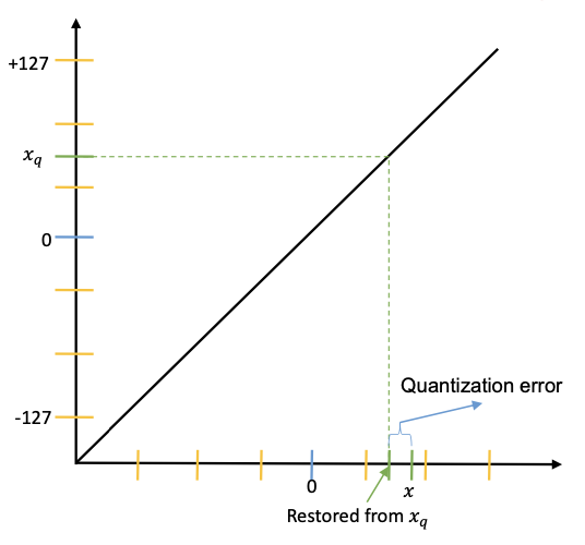
A metric to evaluate the numerical error introduced by quantization.

\[ \mathbf{L}(r, \hat r) \text{ , where } r \approx \hat r = \mathbf{D}(\mathbf{Q}(r)) \]

where \(r\) is the original tensor, \(\hat r = \mathbf{D}(\mathbf{Q}(r))\) is the tensor after quantization and dequantization.

Mean-Square Error (MSE)

The most commonly-used metric for quantization error.

\[ \mathbf{L}(r, \hat r) = \frac{1}{N} \sum_{i=1}^N (r_i - \hat r_i)^2 \]

Other Quantization Error Metrics

• Cosine distance
• Pearson correlation coefficient
• Hessian-guided metric

Fake Quantization/Integer-only Quantization

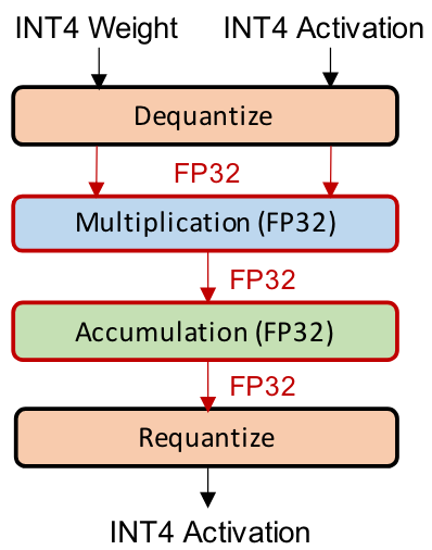
Fake Quantization (Simulated Quantization)

In simulated quantization, the quantized model parameters are stored in low-precision, but the operations (e.g. matrix multiplications and convolutions) are carried out with floating point arithmetic.

Therefore, the quantized parameters need to be dequantized before the floating point operations

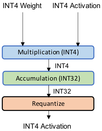
Integer-only Quantization

In integer-only quantization, all the operations are performed using low-precision integer arithmetic.

Hardware-Friendly Design

Dyadic Quantization

A type of integer-only quantization that all of the scaling factors are restricted to be dyadic numbers defined as:

\[ s \approx \frac{b}{2^c} \]

where \(s\) is a floating point number, and \(b\) and \(c\) are integers.

Dyadic quantization can be implemented with only bit shift and integer arithmetic operations, which eliminates overhead of expensive dequantization and requantization.

Power-of-Two Uniform/Scale Quantization (Similar to Dyadic Quantization)

Same concept as dyadic quantization, we replace the numerator \(b\) with \(1\). This approach improves hardware efficiency since it further eliminates the need for the integer multiplier.

\[ s \approx \frac{1}{2^c} \]

:::warning Power-of-Two Uniform/Scale Quantization constrains the scaling factor to a power-of-two value, enabling efficient computation through bit shifts, while Power-of-Two (Logarithmic) Quantization directly quantizes data to power-of-two values, reducing multiplications to simple bitwise operations. :::

Derivation of Quantized MAC

In order to simplify the hardware implementation, we use layerwise symmetric uniform quantization for all layers.

Here are the data types for inputs, weights, biases, outputs, and partial sums:

	input/output	weight	bias/psum
Data type	uint8	int8	int32

Note that the scaling factor of bias is the product of input's scale and weight's scale. And rounding method is truncation instead of round-to-nearest.

\[ \tag{1} \begin{align} \bar x &= \text{clamp} \left( \left\lfloor \frac{x}{s_x} \right\rceil + 128, 0, 255 \right) \in \mathbb{Z}_\text{uint8}^{\dim(x)} \\ \bar w &= \text{clamp} \left( \left\lfloor \frac{w}{s_w} \right\rceil, -128, 127 \right) \in \mathbb{Z}_\text{int8}^{\dim(w)} \\ \bar b &= \text{clamp} \left( \left\lfloor \frac{b}{s_x s_w} \right\rfloor, -2^{31}, 2^{31}-1 \right) \in \mathbb{Z}_\text{int32}^{\dim(b)} \\ \bar y &= \text{clamp} \left( \left\lfloor \frac{y}{s_y} \right\rceil + 128, 0, 255 \right) \in \mathbb{Z}_\text{uint8}^{\dim(y)} \end{align} \]

The notation \(\mathbb{Z}^N\) denotes a vector space of dimension \(N\) where all elements (or components) are integers. See also Cartesian product.

where the scaling factors are calaulated by

\[ \tag{2} \begin{align} s_x = \frac{2 \max(|x_\min|, |x_\max|)|}{255} \in \mathbb{R}_\text{float32} \\ s_w = \frac{2 \max(|w_\min|, |w_\max|)|}{255} \in \mathbb{R}_\text{float32} \\ s_y = \frac{2 \max(|y_\min|, |y_\max|)}{255} \in \mathbb{R}_\text{float32} \end{align} \]

The original values can be approximated by dequantizing the quantized numbers.

\[ \tag{3} \begin{align} x &\approx s_x (\bar x - 128) \\ w &\approx s_w \bar w \\ b &\approx s_x s_w \bar b \\ y &\approx s_y (\bar y - 128) \end{align} \]

Quantized Linear Layer with ReLU

Rectified linear unit (ReLU) is one of the most commonly-used activation functions due to its simplicity.

\[ \text{ReLU}(x) = \max(x, 0) = \begin{cases} x, ~~\text{if} ~ x > 0 \\ 0, ~~\text{otherwise} \end{cases} \]

Linear layer:

\[ y_i = \text{ReLU}(b_i + \sum_j x_j \cdot w_{ji}) \]

\[ s_y (\bar y_i - 128) = \text{ReLU}(s_x s_w (\bar b_i + \sum_j (\bar x_j - 128) \cdot \bar w_{ji})) \]

The scaling factors \(s_x\), \(s_w\), and \(s_y\) are typically in \([0, 1]\), which doesn't affect the result of ReLU.

\[ \tag{5} \bar y_i = \underbrace{ \frac{s_x s_w}{s_y} \overbrace{ \text{ReLU}(\bar b_i + \sum_j (\bar x_j - 128) \cdot \bar w_{ji}) }^{\text{only int32 operations}}}_{\text{float32 operations involved} } + 128 \]

Hardware-Friendly Design

Power-of-Two Quantization

With \(b = 1\) in dyadic quantization, we further get power-of-two quantization:

\[ s \approx \frac{1}{2^c} = 2^{-c} \text{ , where } c \in \mathbb{Z} \]

The matrix multiplication can be approximated as:

\[ \tag{6} \begin{align} \bar y_i &\approx 2^{-(c_x + c_w - c_y)} \text{ReLU}(\bar b_i + \sum_j (\bar x_j - 128) \cdot \bar w_{ji}) + 128 \\ &= \left( \text{ReLU}(\bar b_i + \sum_j (\bar x_j - 128) \cdot \bar w_{ji}) \gg (c_x + c_w - c_y) \right) + 128 \\ \end{align} \]

We can use shifting to replace multiplication and division when applying a scaling factor.

Derivation of Batch Normalization Folding

During inference, batch normalization (BN) can be fused with Conv2d or Linear layers to improve inference efficiency, reduce memory access, and increase computational throughput. This also simplifies the hardware implementation in Lab3 by eliminating the need for separate BN computation. The derivation is as follows.

Consider a batch normalization (BN) layer expressed by the following equation:

\[ \tag{1} z_c = \frac{y_c - \mu_c}{\sqrt{\sigma_c^2 + \epsilon}} \cdot \gamma_c + \beta_c \]

where:

• \(y_c \in \mathbb{R}^{H \times W}\): the \(c\)-th channel of the input tensor (assuming batch size \(N = 1\))
• \(z_c \in \mathbb{R}^{H \times W}\): the \(c\)-th channel of the output tensor (assuming batch size \(N = 1\))
• \(\mu_c \in \mathbb{R}\): mean value of input activations along the \(c\)-th channel
• \(\sigma_c^2 \in \mathbb{R}\): variance of input activations along the \(c\)-th channel
• \(\gamma_c \in \mathbb{R}\) and \(\beta_c \in \mathbb{R}\): BN parameters for the \(c\)-th channel
• \(\epsilon \in \mathbb{R}\): a small value for numerical stability during computation

Expanding Eq. 1, we obtain:

\[ z_c = \left( \frac{\gamma_c}{\sqrt{\sigma_c^2 + \epsilon}} \right) \cdot y_c + \left( \beta_c - \frac{\gamma_c \mu_c}{\sqrt{\sigma_c^2 + \epsilon}} \right) \]

Assuming that the numerical distribution during inference is the same as in the training set, the statistics \(\mu_c\) and \(\sigma_c^2\) obtained during training are considered fixed values during inference. These values can then be fused into the preceding Conv2d or Linear layer.

For example, consider a Linear layer:

\[ \tag{2} y_c = b_c + \sum_i x_i \cdot w_{ic} \]

where the output \(y\) is normalized by BatchNorm to obtain \(z\). Substituting Eq. 2 into Eq. 1:

\[ \begin{align} z_c &= \left( \frac{\gamma_c}{\sqrt{\sigma_c^2 + \epsilon}} \right) \cdot \left( b_c + \sum_i x_i \cdot w_{ic} \right) + \left( \beta_c - \frac{\gamma_c \mu_c}{\sqrt{\sigma_c^2 + \epsilon}} \right) \\ &= \left( \sum_i x_i \cdot \frac{\gamma_cw_{ic}}{\sqrt{\sigma_c^2 + \epsilon}} \right) + \left( \beta_c - \frac{\gamma_c \mu_c}{\sqrt{\sigma_c^2 + \epsilon}} + \frac{\gamma_c b_c}{\sqrt{\sigma_c^2 + \epsilon}} \right) \\ &\triangleq \sum_i x_i \cdot w_{ic}' + b_c' \end{align} \]

After rearranging, we observe that the Linear + BN operation can be expressed as a new Linear operation with updated weights and biases:

\[ \tag{3} \begin{align} w_c' &= \frac{\gamma_c}{\sqrt{\sigma_c^2 + \epsilon}} \cdot w_c \\ b_c' &= \frac{\gamma_c}{\sqrt{\sigma_c^2 + \epsilon}} (b_c - \mu_c) + \beta_c \end{align} \]

Quantization in Practice

In this section, we will demonstrate how to perform quantization with PyTorch framework with a simple yet comprehensive example.

Let's discuss the quantization process using PyTorch step by step:

1. Calibration Data
2. Pre-trained Model
3. Customize Quantization Scheme
4. Operator Fusion
5. Insert Observer
6. Calibration
7. Quantization

1. Calibration Data

During calibration, only a small amount of data is required. Therefore, the batch size is set to 1

dataset = '{DATASET}'
backend = '{Quantization_scheme}'
model_path = 'path/to/your/model'
*_, test_loader = DATALOADERS[dataset](batch_size=1)

2. Pre-trained Model

Load model weights trained from Lab 1.1.

model = network(in_channels, in_size).eval().cpu()
model.load_state_dict(torch.load(model_path))

3. Customize Quantization Scheme

Configure Quantization - model = tq.QuantWrapper(model) Converts the model into a format suitable for quantization.

model = tq.QuantWrapper(model)
model.qconfig = CustomQConfig[{Your_Quantization_Scheme_in_CustomQConfig_class}].value
print(f"Quantization backend: {model.qconfig}")

• QConfig

  qconfig.py

  class CustomQConfig(Enum):
      POWER2 = torch.ao.quantization.QConfig(
          activation=PowerOfTwoObserver.with_args(
              dtype=torch.quint8, qscheme=torch.per_tensor_symmetric
          ),
          weight=PowerOfTwoObserver.with_args(
              dtype=torch.qint8, qscheme=torch.per_tensor_symmetric
          ),
      )
      DEFAULT = None
  

  The torch.ao.quantization.QConfig class helps define custom quantization schemes by specifying:

• How activations should be quantized

• How weights should be quantized

These are parameters tells your custom observer (class PowerOfTwoObserver(...)) how to calculate scale and zero point.

Parameter	Description
dtype=torch.quint8	unsigned 8-bit quantization
dtype=torch.qint8	signed 8-bit quantization
qscheme=torch.per_tensor_symmetric	select symmetric quantization in one tensor
qscheme=torch.per_tensor_affine	select asymmetric quantization in one tensor

4. Operator Fusion

Operator fusion is a technique that combines multiple operations into a single efficient computation to reduce memory overhead and improve execution speed.

Module fusion combines multiple sequential modules (eg: [Conv2d, BatchNorm, ReLU]) into one. Fusing modules means the compiler needs to only run one kernel instead of many; this speeds things up and improves accuracy by reducing quantization error. -- PyTorch

Common fusions include: - Conv2D + BatchNorm + ReLU → Fused into a single Conv2D operation. - Conv2D + ReLU → Fused into a single Conv2D operation. - Linear + ReLU → Fused into a single linear transformation with an activation function.

If you want to performed module fusion to improve performance, you should call the following API before calibration.

tq.fuse_modules(model: nn.Module, modules_to_fuse: list[str], inplace=False) -> nn.Module

You can see the reference for more details.

5. Insert Observer

• tq.prepare(model, inplace=True) : Inserts fake quantization modules to track activations.

  tq.prepare(model, inplace=True)
  

6. Calibration

Define calibration function first:

def calibrate(model, loader, device=DEFAULT_DEVICE):
    model.eval().to(device)
    for x, _ in loader:
        model(x.to(device))
        break

Apply calibration by directly call the above function after inserting the observer via tq.prepare.

calibrate(model, test_loader, "cpu")

This runs one batch of data (previous step) through the model to collect activation statistics.

7. Quantization

Use tq.convert(model.cpu(), inplace=True) to convert the model into a fully-quantized model.

tq.convert(model.cpu(), inplace=True)

Finally, save your quantized model with given filename

save_model({Your Model}, "filename.pt")

Reference

• A Survey of Quantization Methods for Efficient Neural Network Inference
• PyTorch Quantization
• Pooling Methods in Deep Neural Networks, a Review
• NVIDIA Deeplearning Performance Documents

Practice

1. Train a VGG-like Model using CIFAR-10 dataset.

VGG is a classic CNN architecture used in computer vision. Compared to the previous CNNs, it only use 3x3 convolution, making it easy to be implmeneted and supported by existing and customized hardware accelerators.

In this course, we are going to deploy a VGG-like model onto our custom hardware accelerator and complete an end-to-end inference of image recognition. In this lab, students are requested to implement a VGG-like model in PyTorch with only the following operators:

• Conv2d with 3x3 kernel size, stride 1, and padding 1
• Linear
• ReLU
• MaxPool2d with 2x2 kernel size and stride 2
• BatchNorm2d

Layer	Type
Conv1	Conv2D (3 → 64)
MaxPool	2×2 Pooling
Conv2	Conv2D (64 → 192)
MaxPool	2×2 Pooling
Conv3	Conv2D (192 → 384)
Conv4	Conv2D (384 → 256)
Conv5	Conv2D (256 → 256)
MaxPool	2×2 Pooling
Flatten	-
FC6	Linear (256*fmap_size² → 256)
FC7	Linear (256 → 128)
FC8	Linear (128 → num_classes)

Students are required to design and train your model with only allowed operators using as few parameters as possible while ensuring the accuracy greater than 80%. You can use any training techniques and adjust the hyperparameters (e.g. learning rate tuning, optimizer, etc.) to achieve this goal.

For full precision model, your model should achive the following metrics: - top-1 accuracy remains above 80% on the CIFAR-10 classification task

2. Quantize the VGG-like Model as INT8 Precision

Then, quantize the model to INT8 precision while preserving a high level of accuracy compared to the full-precision model.

Quantization scheme

Use the power-of-two uniform/scale, symmetric quantization we previously-mentioned to quantize your model. - Complete the QConfig observer setup for Post-Training Quantization (PTQ) calibration. - Reference: PyTorch QConfig documents

For quantized model, your model should achive the following metrics:

• model size \(<\) 4MB
• top-1 accuracy on CIFAR-10 \(\ge\) 80%
• accuracy drop \(\le\) 1% compared to your full-precision model